Subcritical Swift-Hohenberg equation (SH23)

Overview

The Swift-Hohenberg equation is the canonical model of pattern formation near a finite-wavenumber instability, introduced by Swift and Hohenberg in 1977 for Rayleigh-Bénard convection. Its quadratic-cubic (subcritical) variant, commonly called SH23, reads

\[u_t = r u - \left(1 + \partial_x^2\right)^2 u + b u^2 - u^3,\]

$u(x,t)$: scalar field (e.g. the deviation of the temperature from the conducting state)
$r$: bifurcation parameter (distance from the onset of the instability)
$b$: strength of the quadratic nonlinearity, which breaks the $u \mapsto -u$ symmetry

Some properties

Linear stability: a Fourier mode $e^{ikx}$ grows at the rate $\sigma(k) = r - (1-k^2)^2$. The trivial state $u \equiv 0$ is linearly stable for $r < 0$ and loses stability at $r = 0$ to the critical wavenumber $k_c = 1$. Modes away from $k_c$ are strongly damped ($\sigma \sim -k^4$).
Subcriticality and bistability: for $b^2 > 27/38$ the bifurcation at $r=0$ is subcritical. A finite-amplitude periodic pattern then coexists with the stable trivial state for $r_{\mathrm{sn}} < r < 0$, where $r_{\mathrm{sn}}$ is the saddle-node of the periodic branch ($r_{\mathrm{sn}} \approx -0.37$ for $b = 1.8$ and wavenumber $k=1$). In this window the basin of attraction of $u \equiv 0$ is bounded by the stable manifolds of unstable (lower-branch) states, which makes the model a test case for methods that estimate regions of attraction.
Localized states: inside the bistable window, spatially localized patches of pattern exist and organize in the snaking bifurcation diagram described by Burke and Knobloch (2006). On domains of only a few wavelengths these states have little room and the dynamics is dominated by the periodic pattern.
Gradient flow: SH23 is the $L_2$-gradient flow of the Lyapunov functional
\[E(u) = \int \left( -\frac{r}{2}u^2 + \frac{1}{2}\left[(1+\partial_x^2)u\right]^2 - \frac{b}{3}u^3 + \frac{1}{4}u^4 \right) dx,\]
so every bounded trajectory converges to a steady state.

Model

Expanding the linear operator as $(r-1) - 2\partial_x^2 - \partial_x^4$, the semi-discrete SH23 equation is a linear-quadratic-cubic model:

\[\dot{\mathbf{u}}(t) = \mathbf{Au}(t) + \mathbf{F}(\mathbf{u}(t) \oslash \mathbf{u}(t)) + \mathbf{E}(\mathbf{u}(t) \oslash \mathbf{u}(t) \oslash \mathbf{u}(t)) + \mathbf{Bw}(t)\]

where

$\mathbf{u}\in\mathbb{R}^N$: the state vector
$\mathbf{w}\in\mathbb{R}^m$: the input vector (Dirichlet boundary values)
$\mathbf{A}\in\mathbb{R}^{N\times N}$: the linear state matrix, a symmetric pentadiagonal matrix from second-order central differences
$\mathbf{F}\in\mathbb{R}^{N\times N(N+1)/2}$: the quadratic state matrix without redundancy (the $bu^2$ term)
$\mathbf{E}\in\mathbb{R}^{N\times N(N+1)(N+2)/6}$: the cubic state matrix without redundancy (the $-u^3$ term)
$\mathbf{B}\in\mathbb{R}^{N\times m}$: the control input matrix

The model parameters are passed as params=Dict(:r => ..., :b => ...).

Boundary conditions

:periodic: $\mathbf{A}$ is a circulant matrix. Use Δx = (Ω[2]-Ω[1])/Nx so that the discrete period equals the domain length; since the dynamics selects the wavenumber $k_c = 1$, a domain of length $2\pi m$ holds exactly $m$ critical wavelengths.
:dirichlet: hinged (simply supported) conditions $u = g$ and $u_{xx} = 0$. As in the other Dirichlet models of this package, the boundary values $g_L, g_R$ sit at ghost nodes one grid spacing outside xspan; the condition $u_{xx} = 0$ fixes the second ghost node by reflection, $u_{-1} = 2g_L - u_1$. With $g_L = g_R = 0$ the operator $\mathbf{A}$ is symmetric and diagonalized by the discrete sine transform. The two columns of $\mathbf{B}$ carry $g_L$ and $g_R$.

Numerical Integration

For the numerical integration we consider two methods:

Semi-Implicit Crank-Nicolson (SICN)
Crank-Nicolson Adams-Bashforth (CNAB)

Both treat the stiff linear operator $\mathbf{A}$ with Crank-Nicolson and the reaction term $\mathbf{N}(\mathbf{u}) = \mathbf{F}\mathbf{u}^{\langle 2\rangle} + \mathbf{E}\mathbf{u}^{\langle 3\rangle}$ explicitly.

SICN:

\[\mathbf{u}(t_{k+1}) = \left(\mathbf{I}-\frac{\Delta t}{2}\mathbf{A}\right)^{-1} \left\{ \left( \mathbf{I} + \frac{\Delta t}{2}\mathbf{A} \right)\mathbf{u}(t_k) + \Delta t\,\mathbf{N}(\mathbf{u}(t_k)) + \frac{\Delta t}{2} \mathbf{B}\left[ \mathbf{w}(t_{k+1}) + \mathbf{w}(t_k) \right]\right\}\]

CNAB:

If $k=1$ the SICN step is used. If $k\geq 2$

\[\mathbf{u}(t_{k+1}) = \left(\mathbf{I}-\frac{\Delta t}{2}\mathbf{A}\right)^{-1} \left\{ \left( \mathbf{I} + \frac{\Delta t}{2}\mathbf{A} \right)\mathbf{u}(t_k) + \frac{3\Delta t}{2}\mathbf{N}(\mathbf{u}(t_k)) - \frac{\Delta t}{2}\mathbf{N}(\mathbf{u}(t_{k-1})) + \frac{\Delta t}{2} \mathbf{B}\left[ \mathbf{w}(t_{k+1}) + \mathbf{w}(t_k) \right]\right\}\]

where $\mathbf{u}^{\langle 2 \rangle}=\mathbf{u} \oslash \mathbf{u}$ and $\mathbf{u}^{\langle 3 \rangle}=\mathbf{u} \oslash \mathbf{u} \oslash \mathbf{u}$.

The fast integrator integrate_model_fast uses the same schemes with a pre-built solver from build_fast_solver. Because $\mathbf{A}$ is pentadiagonal, the tridiagonal solver does not apply: periodic boundaries use the FFT-based FastCirculant1DSolver, and Dirichlet boundaries use FastDenseSolver, which eigendecomposes the symmetric operator once and caches $(\mathbf{I}-\frac{\Delta t}{2}\mathbf{A})^{-1}$.

!!! Note Please go over the derivations in 1D heat equation and Kuramoto-Sivashinsky equation for details on how to construct the second- and fourth-order difference operators.

Example

using CairoMakie
using LinearAlgebra
using PolynomialModelReductionDataset
const pomoreda = PolynomialModelReductionDataset

# Setup: four critical wavelengths on a periodic domain, inside the bistable window
Ω = (0.0, 8π)
T = (0.0, 50.0)
Nx = 2^7
dt = 1e-2
sh = pomoreda.SwiftHohenbergModel(
    spatial_domain=Ω, time_domain=T, Δx=(Ω[2]-Ω[1])/Nx, Δt=dt,
    params=Dict(:r => -0.2, :b => 1.8), BC=:periodic
)
DS = 10
x = sh.xspan

# Operators and fast solver
A, F, E = sh.finite_diff_model(sh, sh.params)
solver = pomoreda.build_fast_solver(sh, sh.params; scheme=:CN)

# Two perturbations of the critical mode on either side of the threshold
sh.IC = 0.2 * cos.(x)
U_small = pomoreda.integrate_model_fast(sh, solver, sh.tspan, sh.IC;
                                        quadratic_matrix=F, cubic_matrix=E, integrator_type=:CNAB)
sh.IC = 1.0 * cos.(x)
U_large = pomoreda.integrate_model_fast(sh, solver, sh.tspan, sh.IC;
                                        quadratic_matrix=F, cubic_matrix=E, integrator_type=:CNAB)

fig = Figure(size=(900, 400))
crange = (-1.5, 1.5)
ax1 = Axis(fig[1, 1], xlabel=L"x", ylabel=L"t", title="Small perturbation: decays to 0")
heatmap!(ax1, x, sh.tspan[1:DS:end], U_small[:, 1:DS:end], colorrange=crange, colormap=:balance)
ax2 = Axis(fig[1, 2], xlabel=L"x", ylabel=L"t", title="Large perturbation: saturates on the pattern")
hm = heatmap!(ax2, x, sh.tspan[1:DS:end], U_large[:, 1:DS:end], colorrange=crange, colormap=:balance)
Colorbar(fig[1, 3], hm)
fig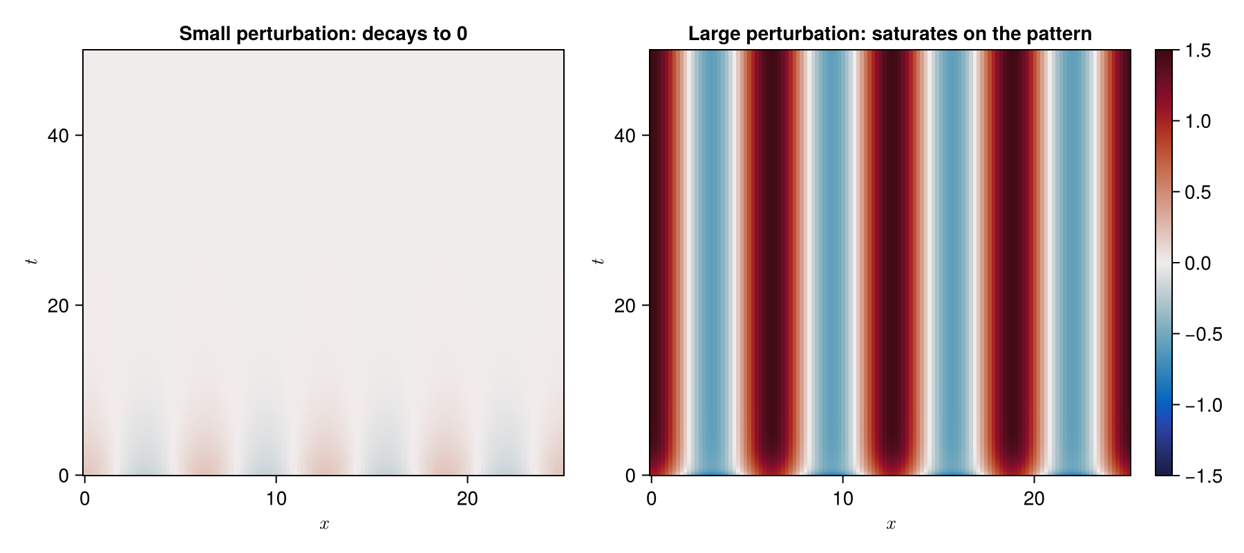

API

PolynomialModelReductionDataset.SwiftHohenberg.SwiftHohenbergModel — Type

mutable struct SwiftHohenbergModel <: AbstractModel

Subcritical (quadratic-cubic) Swift-Hohenberg equation model, commonly called SH23:

\[\frac{\partial u}{\partial t} = r u - \left(1 + \frac{\partial^2}{\partial x^2}\right)^2 u + b u^2 - u^3\]

where $u$ is the state variable, $r$ is the bifurcation (control) parameter, and $b$ is the quadratic coefficient. Expanding the linear operator,

\[\frac{\partial u}{\partial t} = (r-1) u - 2\frac{\partial^2 u}{\partial x^2} - \frac{\partial^4 u}{\partial x^4} + b u^2 - u^3,\]

so the semi-discrete model is linear-quadratic-cubic in the state. The linear growth rate of a Fourier mode $e^{ikx}$ is $r - (1-k^2)^2$, so the trivial state is linearly stable for $r<0$. For $b^2 > 27/38$ the pattern-forming bifurcation at $r=0$ is subcritical: a finite-amplitude periodic pattern coexists with the stable trivial state for $r_{\mathrm{sn}} < r < 0$, and the basin of $u \equiv 0$ is bounded by the stable manifolds of the unstable (lower-branch) states. For $b=1.8$ the saddle-node of the $k=1$ periodic branch is at $r_{\mathrm{sn}} \approx -0.37$.

Fields

spatial_domain::Tuple{Real,Real}: spatial domain
time_domain::Tuple{Real,Real}: temporal domain
param_domain::Dict{Symbol,Tuple{Real,Real}}: parameter domain
Δx::Real: spatial grid size
Δt::Real: temporal step size
xspan::Vector{<:Real}: spatial grid points
tspan::Vector{<:Real}: temporal points
params::Dict{Symbol,Union{Real,AbstractArray{<:Real}}}: parameters (:r bifurcation parameter, :b quadratic coefficient)
spatial_dim::Int: spatial dimension
time_dim::Int: temporal dimension
param_dim::Dict{Symbol,Int}: parameter dimension
IC::AbstractArray{<:Real}: initial condition
BC::Symbol: boundary condition (:periodic or :dirichlet)
finite_diff_model::Function: model using Finite Difference
integrate_model::Function: integrator using Crank-Nicolson (linear) Explicit (nonlinear) method