Kawahara Equation

Overview

The Kawahara equation (also known as the dispersively-modified Kuramoto-Sivashinsky equation or Benney-Lin equation) is a nonlinear partial differential equation that describes the evolution of certain physical systems, particularly in fluid dynamics and plasma physics. It extends the Kuramoto-Sivashinsky equation by including higher-order dispersion terms.

The equation can be written in several forms depending on which dispersion terms are included:

First-order dispersion:

\[\frac{\partial u}{\partial t} = -\mu\frac{\partial^4 u}{\partial x^4} - \frac{\partial^2 u}{\partial x^2} - u\frac{\partial u}{\partial x} - \delta\frac{\partial u}{\partial x}\]

Third-order dispersion:

\[\frac{\partial u}{\partial t} = -\mu\frac{\partial^4 u}{\partial x^4} - \frac{\partial^2 u}{\partial x^2} - u\frac{\partial u}{\partial x} - \delta\frac{\partial^3 u}{\partial x^3}\]

Fifth-order dispersion:

\[\frac{\partial u}{\partial t} = -\mu\frac{\partial^4 u}{\partial x^4} - \frac{\partial^2 u}{\partial x^2} - u\frac{\partial u}{\partial x} - \nu\frac{\partial^5 u}{\partial x^5}\]

Combined dispersion (third and fifth order):

\[\frac{\partial u}{\partial t} = -\mu\frac{\partial^4 u}{\partial x^4} - \frac{\partial^2 u}{\partial x^2} - u\frac{\partial u}{\partial x} - \delta\frac{\partial^3 u}{\partial x^3} - \nu\frac{\partial^5 u}{\partial x^5}\]

where:

• $u(x, t)$ is the state variable
• $\mu$ is the viscosity coefficient (fourth-order diffusion)
• $\delta$ is the first-order or third-order dispersion coefficient
• $\nu$ is the fifth-order dispersion coefficient
• The term $-u\frac{\partial u}{\partial x}$ represents nonlinear advection

The Kawahara equation exhibits a rich variety of spatiotemporal behaviors including traveling waves, solitary waves, and chaotic dynamics. The higher-order dispersion terms provide additional stabilization mechanisms compared to the standard Kuramoto-Sivashinsky equation.

Model

For our analysis, we discretize the original PDE and separate the system into linear and nonlinear components:

\[\dot{\mathbf{u}}(t) = \mathbf{A}\mathbf{u}(t) + \mathbf{F}\mathbf{u}^{\langle 2\rangle}(t)\]

where:

• $\mathbf{A}$ is the linear operator (containing diffusion, anti-diffusion, and dispersion terms)
• $\mathbf{F}$ is the quadratic operator (for the nonlinear advection)
• $\mathbf{u}^{\langle 2\rangle}$ represents the quadratic states (non-redundant)

Conservation Forms

The implementation supports three different conservation forms for the nonlinear term:

1. Non-Conservative (NC): $-u\frac{\partial u}{\partial x}$
2. Conservative (C): $-\frac{1}{2}\frac{\partial (u^2)}{\partial x}$
3. Energy-Preserving (EP): A skew-symmetric discretization that preserves discrete energy

The choice of conservation form affects the numerical properties and long-term behavior of the solution.

Numerical Integration

We integrate the Kawahara model using the Crank-Nicolson Adams-Bashforth (CNAB) method, treating the linear terms implicitly and the nonlinear term explicitly:

\[\mathbf{u}(t_{k+1}) = \begin{cases} \left(\mathbf{I} - \frac{\Delta t}{2}\mathbf{A}\right)^{-1}\left[\left(\mathbf{I} + \frac{\Delta t}{2}\mathbf{A}\right)\mathbf{u}(t_k) + \Delta t\mathbf{F}\left(\mathbf{u}(t_k)\right)^{\langle 2\rangle}\right] & k = 1 \\[0.3cm] \left(\mathbf{I} - \frac{\Delta t}{2}\mathbf{A}\right)^{-1}\left[\left(\mathbf{I} + \frac{\Delta t}{2}\mathbf{A}\right)\mathbf{u}(t_k) + \frac{3\Delta t}{2}\mathbf{F}\left(\mathbf{u}(t_k)\right)^{\langle 2\rangle} - \frac{\Delta t}{2}\mathbf{F}\left(\mathbf{u}(t_{k-1})\right)^{\langle 2\rangle}\right] & k \geq 2 \end{cases}\]

This scheme provides second-order accuracy in time and good stability properties for the stiff linear terms.

Finite Difference Model

We discretize the spatial derivatives using centered finite differences. The discretization depends on the dispersion order:

For first-order dispersion ($\delta \partial_x u$):

\[u_x \approx \frac{1}{2\Delta x}(u_{n+1} - u_{n-1})\]

For third-order dispersion ($\delta \partial_x^3 u$):

\[u_{xxx} \approx \frac{1}{2\Delta x^3}(u_{n+2} - 2u_{n+1} + 2u_{n-1} - u_{n-2})\]

For fifth-order dispersion ($\nu \partial_x^5 u$):

\[u_{xxxxx} \approx \frac{1}{2\Delta x^5}(u_{n+3} - 4u_{n+2} + 5u_{n+1} - 5u_{n-1} + 4u_{n-2} - u_{n-3})\]

For the fourth-order diffusion:

\[u_{xxxx} \approx \frac{1}{\Delta x^4}(u_{n+2} - 4u_{n+1} + 6u_n - 4u_{n-1} + u_{n-2})\]

For the anti-diffusion:

\[u_{xx} \approx \frac{1}{\Delta x^2}(u_{n+1} - 2u_n + u_{n-1})\]

The linear operator $\mathbf{A}$ combines all these terms into a sparse matrix with periodic boundary conditions, resulting in a circulant-like structure.

The quadratic operator $\mathbf{F}$ discretizes the nonlinear advection term according to the chosen conservation form.

Example - Third-order Dispersion

using CairoMakie
using LinearAlgebra
using PolynomialModelReductionDataset: KawaharaModel

# Settings
Ω = (0.0, 50.0)
dt = 0.01
N = 256
kawahara = KawaharaModel(
    spatial_domain=Ω, time_domain=(0.0, 150.0),
    params=Dict(:mu => 1.0, :delta => 0.15, :nu => 0.0),
    dispersion_order=3,
    conservation_type=:C,
    Δx=(Ω[2] - 1/N)/N, Δt=dt
)
DS = 100
L = kawahara.spatial_domain[2]

# Initial condition
a = 1.0
b = 0.1
u0 = a*cos.((2*π*kawahara.xspan)/L) + b*cos.((4*π*kawahara.xspan)/L)

# Operators
A, F = kawahara.finite_diff_model(kawahara, kawahara.params[:mu], kawahara.params[:delta])

# Integrate
U = kawahara.integrate_model(
    kawahara.tspan, u0, nothing;
    linear_matrix=A, quadratic_matrix=F, const_stepsize=true
)

# Heatmap
fig1, ax, hm = CairoMakie.heatmap(kawahara.tspan[1:DS:end], kawahara.xspan, U[:, 1:DS:end]')
ax.xlabel = L"t"
ax.ylabel = L"x"
CairoMakie.Colorbar(fig1[1, 2], hm)
fig1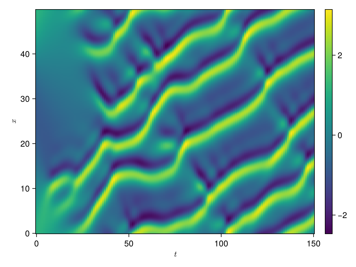

# Surface plot
fig2, _, sf = CairoMakie.surface(kawahara.xspan, kawahara.tspan[1:DS:end], U[:, 1:DS:end],
    axis=(type=Axis3, xlabel=L"x", ylabel=L"t", zlabel=L"u(x,t)"))
CairoMakie.Colorbar(fig2[1, 2], sf)
fig2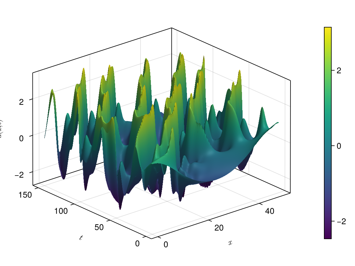

Example - Fifth-order Dispersion

using CairoMakie
using LinearAlgebra
using PolynomialModelReductionDataset: KawaharaModel

# Settings
Ω = (0.0, 50.0)
dt = 0.01
N = 256
kawahara = KawaharaModel(
    spatial_domain=Ω, time_domain=(0.0, 150.0),
    params=Dict(:mu => 1.0, :delta => 0.0, :nu => 0.05),
    dispersion_order=5,
    conservation_type=:EP,
    Δx=(Ω[2] - 1/N)/N, Δt=dt
)
DS = 100
L = kawahara.spatial_domain[2]

# Initial condition
a = 1.0
b = 0.1
u0 = a*cos.((2*π*kawahara.xspan)/L) + b*cos.((4*π*kawahara.xspan)/L)

# Operators
A, F = kawahara.finite_diff_model(kawahara, kawahara.params[:mu], kawahara.params[:delta], kawahara.params[:nu])

# Integrate
U = kawahara.integrate_model(
    kawahara.tspan, u0, nothing;
    linear_matrix=A, quadratic_matrix=F, const_stepsize=true
)

# Heatmap
fig3, ax, hm = CairoMakie.heatmap(kawahara.tspan[1:DS:end], kawahara.xspan, U[:, 1:DS:end]')
ax.xlabel = L"t"
ax.ylabel = L"x"
CairoMakie.Colorbar(fig3[1, 2], hm)
fig3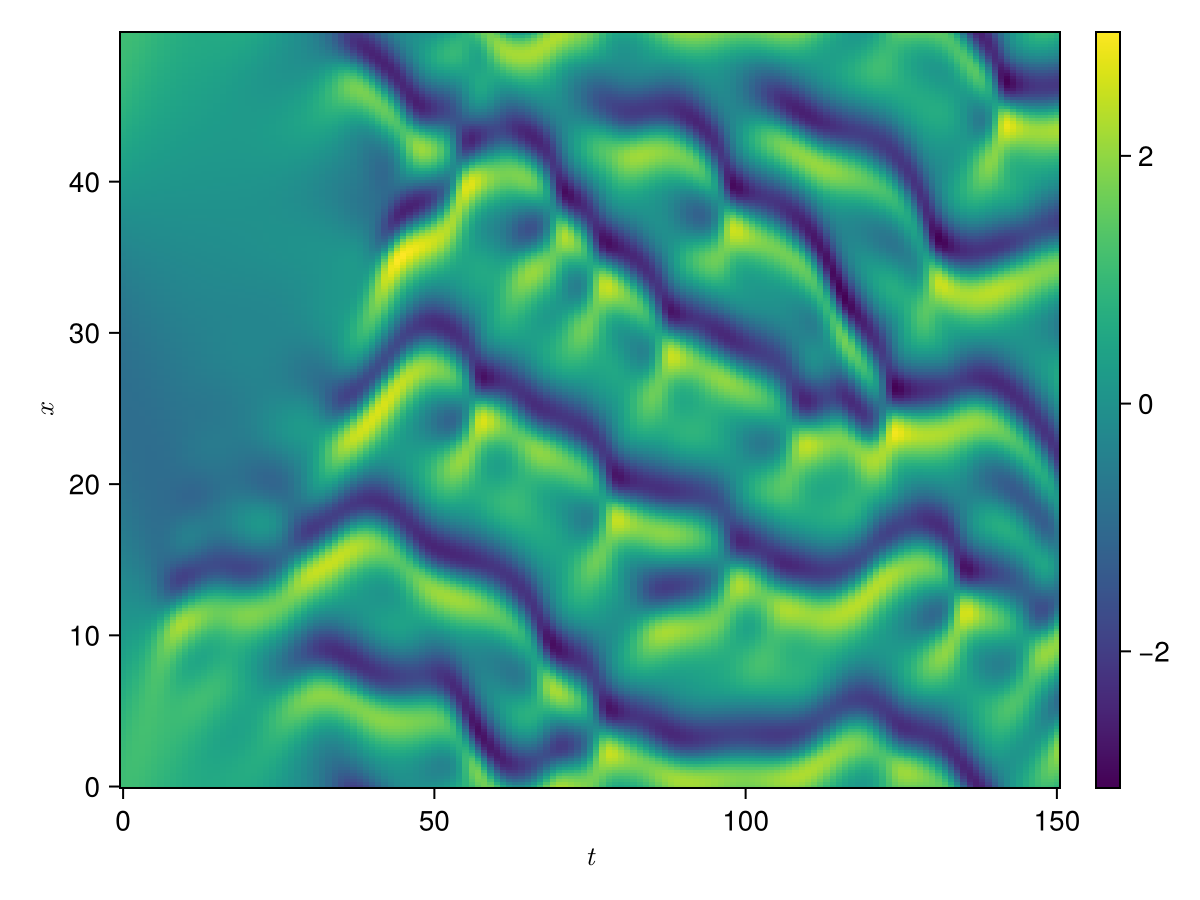

API

mutable struct KawaharaModel <: AbstractModel

Kawahara or Dispersively-Modified Kuramoto-Sivashinsky Equation model

finite_diff_model(model, μ, δ)
finite_diff_model(model, μ, δ, ν)

finite_diff_periodic_conservative_model(N, Δx, μ, δ, ord)
finite_diff_periodic_conservative_model(N, Δx, μ, δ, ord, ν)

finite_diff_periodic_energy_preserving_model(
    N,
    Δx,
    μ,
    δ,
    ord
)
finite_diff_periodic_energy_preserving_model(
    N,
    Δx,
    μ,
    δ,
    ord,
    ν
)

finite_diff_periodic_nonconservative_model(N, Δx, μ, δ, ord)
finite_diff_periodic_nonconservative_model(
    N,
    Δx,
    μ,
    δ,
    ord,
    ν
)

integrate_finite_diff_model(tdata, IC, args; kwargs...)