2D Allen-Cahn Equation

Overview

The Allen-Cahn equation is a reaction-diffusion equation that was originally introduced to describe phase separation in multi-component alloy systems. It models the evolution of a non-conserved order parameter and is widely used to study interface dynamics, pattern formation, and phase transitions.

The 2D Allen-Cahn equation is given by:

\[\frac{\partial u}{\partial t} = \mu\left(\frac{\partial^2 u}{\partial x^2} + \frac{\partial^2 u}{\partial y^2}\right) - \epsilon(u^3 - u)\]

where:

• $u(x, y, t)$ is the order parameter (e.g., concentration or phase indicator)
• $\mu$ is the diffusion coefficient (also called mobility parameter)
• $\epsilon$ is the nonlinear coefficient that determines the interface width
• $x, y$ are spatial coordinates
• $t$ is time

The cubic nonlinearity $-\epsilon(u^3 - u)$ creates a double-well potential that drives the system toward two stable phases (typically represented by $u \approx \pm 1$), while the diffusion term smooths interfaces between these phases.

Model

For our numerical implementation, we discretize the PDE and separate the system into linear and nonlinear components:

\[\dot{\mathbf{u}}(t) = \mathbf{A}\mathbf{u}(t) + \mathbf{E}\mathbf{u}^{\langle 3\rangle}(t) + \mathbf{B}\mathbf{w}(t)\]

where:

• $\mathbf{A}$ is the linear operator (containing diffusion and linear reaction terms)
• $\mathbf{E}$ is the cubic operator (for the $u^3$ term)
• $\mathbf{u}^{\langle 3\rangle}$ represents the cubic states (non-redundant)
• $\mathbf{B}$ is the control/input matrix (for boundary conditions)
• $\mathbf{w}(t)$ represents boundary inputs (if applicable)

Numerical Integration

We integrate the Allen-Cahn model using semi-implicit time-stepping schemes that treat the linear diffusion term implicitly and the nonlinear term explicitly. Two methods are available:

Semi-Implicit Crank-Nicolson (SICN)

\[\frac{\mathbf{u}(t_{k+1}) - \mathbf{u}(t_k)}{\Delta t} = \mathbf{A}\left(\frac{\mathbf{u}(t_{k+1}) + \mathbf{u}(t_k)}{2}\right) + \mathbf{E}\left(\mathbf{u}(t_k)\right)^{\langle 3\rangle}\]

Crank-Nicolson Adams-Bashforth (CNAB)

\[\frac{\mathbf{u}(t_{k+1}) - \mathbf{u}(t_k)}{\Delta t} = \mathbf{A}\left(\frac{\mathbf{u}(t_{k+1}) + \mathbf{u}(t_k)}{2}\right) + \frac{3}{2}\mathbf{E}\left(\mathbf{u}(t_k)\right)^{\langle 3\rangle} - \frac{1}{2}\mathbf{E}\left(\mathbf{u}(t_{k-1})\right)^{\langle 3\rangle}\]

Both methods provide second-order accuracy in time and maintain good stability properties for stiff systems.

Finite Difference Model

The spatial discretization follows the same approach as the 2D Heat equation for the diffusion terms. The domain is discretized with $N_x$ and $N_y$ grid points in the $x$ and $y$ directions respectively.

For periodic boundary conditions, we construct circulant matrices for each direction:

\[\mathbf{A}_x \in \mathbb{R}^{N_x \times N_x}, \quad \mathbf{A}_y \in \mathbb{R}^{N_y \times N_y}\]

The 2D linear operator is then constructed using the Kronecker sum:

\[\mathbf{A} = \mathbf{A}_y \otimes \mathbf{I}_{N_x} + \mathbf{I}_{N_y} \otimes \mathbf{A}_x\]

where $\mathbf{I}$ denotes the identity matrix.

The cubic operator $\mathbf{E}$ is constructed to map the non-redundant cubic monomials to the state derivatives. For a system with $N_{total} = N_x \times N_y$ degrees of freedom, the cubic monomial space has dimension $S = N_{total}(N_{total}+1)(N_{total}+2)/6$.

For Dirichlet boundary conditions, we additionally construct a control matrix $\mathbf{B}$ that applies boundary values at the appropriate grid points (left, right, bottom, top boundaries).

Example - Periodic BC

In this example, we demonstrate phase separation from a star-shaped initial condition with periodic boundary conditions.

using CairoMakie
using LinearAlgebra
using PolynomialModelReductionDataset: AllenCahn2DModel
using UniqueKronecker: invec

# Setup
Ω = ((0.0, 1.0), (0.0, 1.0))
Nx = 2^5
Ny = 2^5
allencahn2d = AllenCahn2DModel(
    spatial_domain=Ω, time_domain=(0,1.0),
    Δx=(Ω[1][2] + 1/Nx)/Nx, Δy=(Ω[2][2] + 1/Ny)/Ny, Δt=1e-3,
    params=Dict(:μ => 1e-2, :ϵ => 1.0), BC=(:periodic, :periodic)
)

# Star-shaped initial condition (centered at 0.5, 0.5)
xgrid0 = allencahn2d.xspan
ygrid0 = allencahn2d.yspan
X_grid = repeat(xgrid0', length(ygrid0), 1)    # size (Ny, Nx)
Y_grid = repeat(ygrid0, 1, length(xgrid0))     # size (Ny, Nx)

# Compute angle θ for each grid point
θ = atan.(Y_grid .- 0.5, X_grid .- 0.5)

# Star radius with 6 points
r_star = 0.25 .+ 0.1 .* cos.(6 .* θ)

# Distance from center
r_actual = sqrt.((X_grid .- 0.5).^2 .+ (Y_grid .- 0.5).^2)

# Diffuse interface parameter
ϵ = allencahn2d.params[:ϵ]

# Star initial condition using tanh
ux0 = tanh.((r_star .- r_actual) ./ sqrt(2 * ϵ))
allencahn2d.IC = vec(ux0)

# Operators
A, E = allencahn2d.finite_diff_model(allencahn2d, allencahn2d.params)

# Integrate
U = allencahn2d.integrate_model(
    allencahn2d.tspan, allencahn2d.IC;
    linear_matrix=A, cubic_matrix=E,
    system_input=false, const_stepsize=true,
)

# Visualize initial condition
U2d = invec.(eachcol(U), allencahn2d.spatial_dim...)
fig1 = Figure()
ax1 = Axis(fig1[1, 1], xlabel="x", ylabel="y", aspect=DataAspect(), title="Initial Condition")
hm1 = heatmap!(ax1, allencahn2d.xspan, allencahn2d.yspan, U2d[1])
Colorbar(fig1[1, 2], hm1)
fig1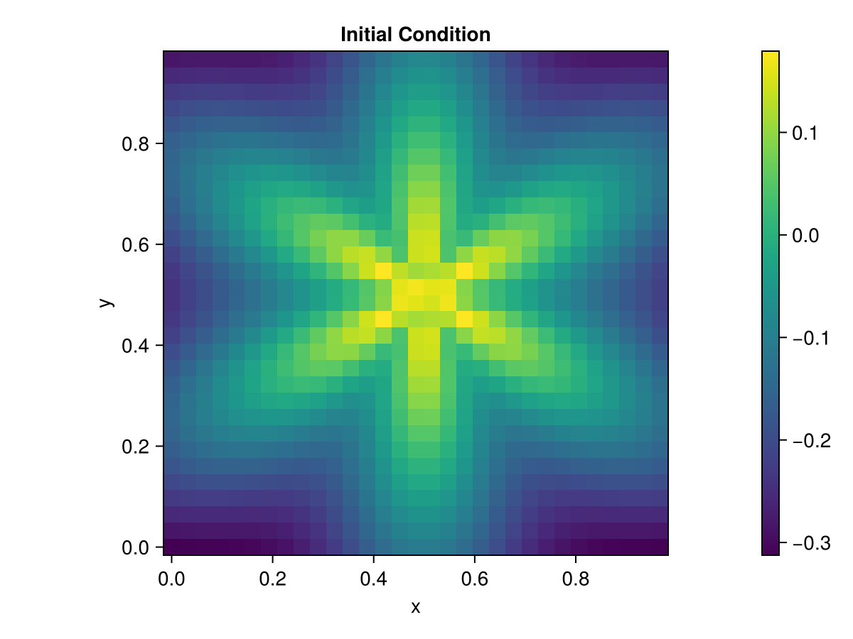

# Visualize final state
fig2 = Figure()
ax2 = Axis(fig2[1, 1], xlabel="x", ylabel="y", aspect=DataAspect(), title="Final State")
hm2 = heatmap!(ax2, allencahn2d.xspan, allencahn2d.yspan, U2d[end])
Colorbar(fig2[1, 2], hm2)
fig2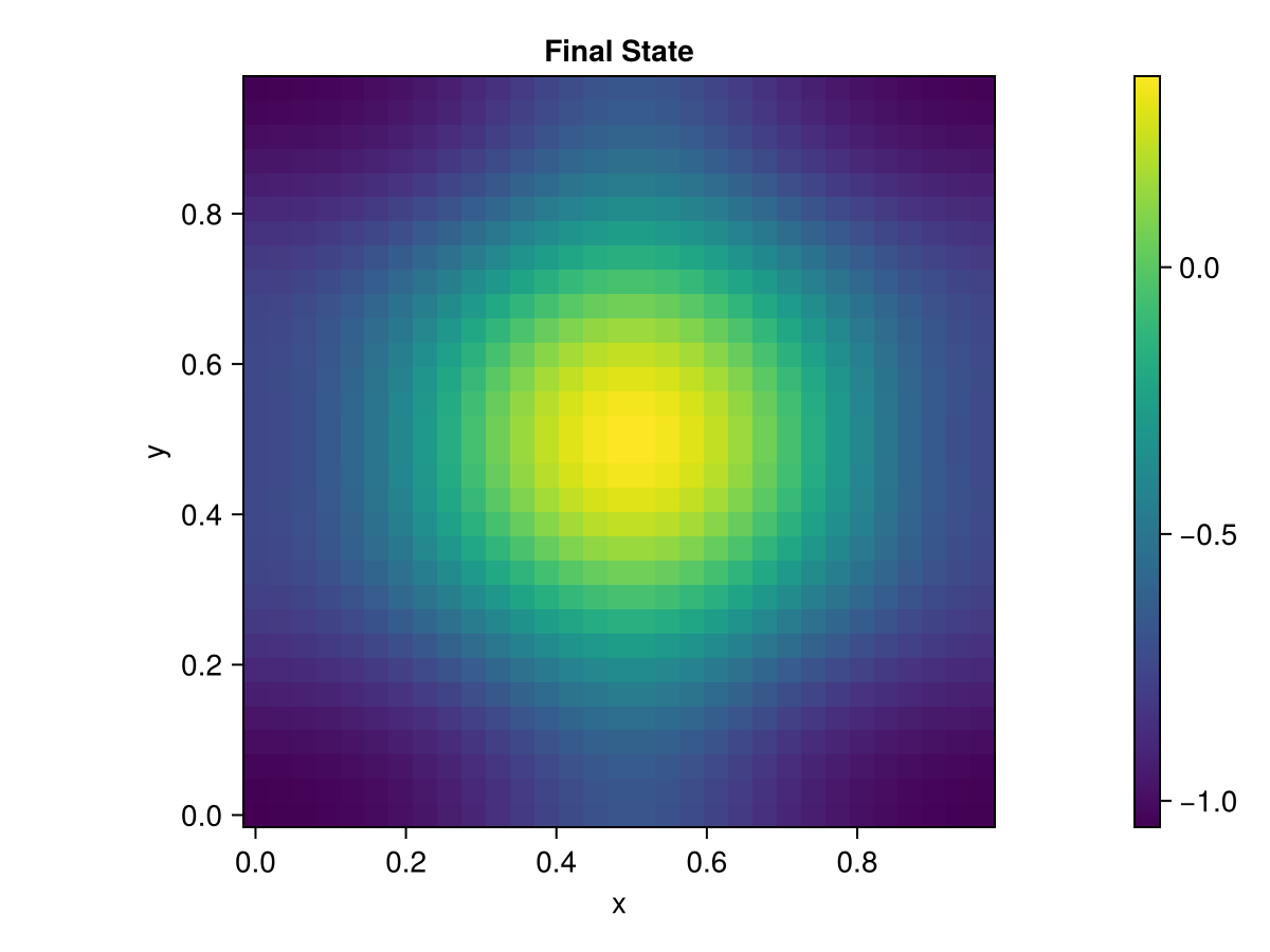

Example - Dirichlet BC

In this example, we demonstrate phase evolution with Dirichlet boundary conditions that fix the phases at the boundaries.

using CairoMakie
using LinearAlgebra
using PolynomialModelReductionDataset: AllenCahn2DModel
using UniqueKronecker: invec

# Setup
Ω = ((0.0, 1.0), (0.0, 1.0))
Nx = 2^5
Ny = 2^5
allencahn2d = AllenCahn2DModel(
    spatial_domain=Ω, time_domain=(0,1.0),
    Δx=(Ω[1][2] + 1/Nx)/Nx, Δy=(Ω[2][2] + 1/Ny)/Ny, Δt=1e-3,
    params=Dict(:μ => 0.001, :ϵ => 1.0), BC=(:dirichlet, :dirichlet)
)

# Initial condition
xg = allencahn2d.xspan
yg = allencahn2d.yspan
X = repeat(xg', length(yg), 1)
Y = repeat(yg, 1, length(xg))

ux0 = 0.1 .* sin.(2π .* X) .* cos.(2π .* Y)
allencahn2d.IC = vec(ux0)

# Dirichlet boundary values: [left, right, bottom, top]
Ubc_vals = [1.0, 1.0, -1.0, -1.0]
Ubc = repeat(reshape(Ubc_vals, 4, 1), 1, allencahn2d.time_dim)

# Operators
A, E, B = allencahn2d.finite_diff_model(allencahn2d, allencahn2d.params)

# Integrate
U = allencahn2d.integrate_model(
    allencahn2d.tspan, allencahn2d.IC, Ubc;
    linear_matrix=A, cubic_matrix=E, control_matrix=B,
    system_input=true, const_stepsize=true,
    integrator_type=:SICN,
)

# Visualize
U2d = invec.(eachcol(U), allencahn2d.spatial_dim...)
fig3 = Figure()
ax3 = Axis3(fig3[1, 1], xlabel="x", ylabel="y", zlabel="u(x,y,t)", title="Final State")
sf = surface!(ax3, allencahn2d.xspan, allencahn2d.yspan, U2d[end])
Colorbar(fig3[1, 2], sf)
fig3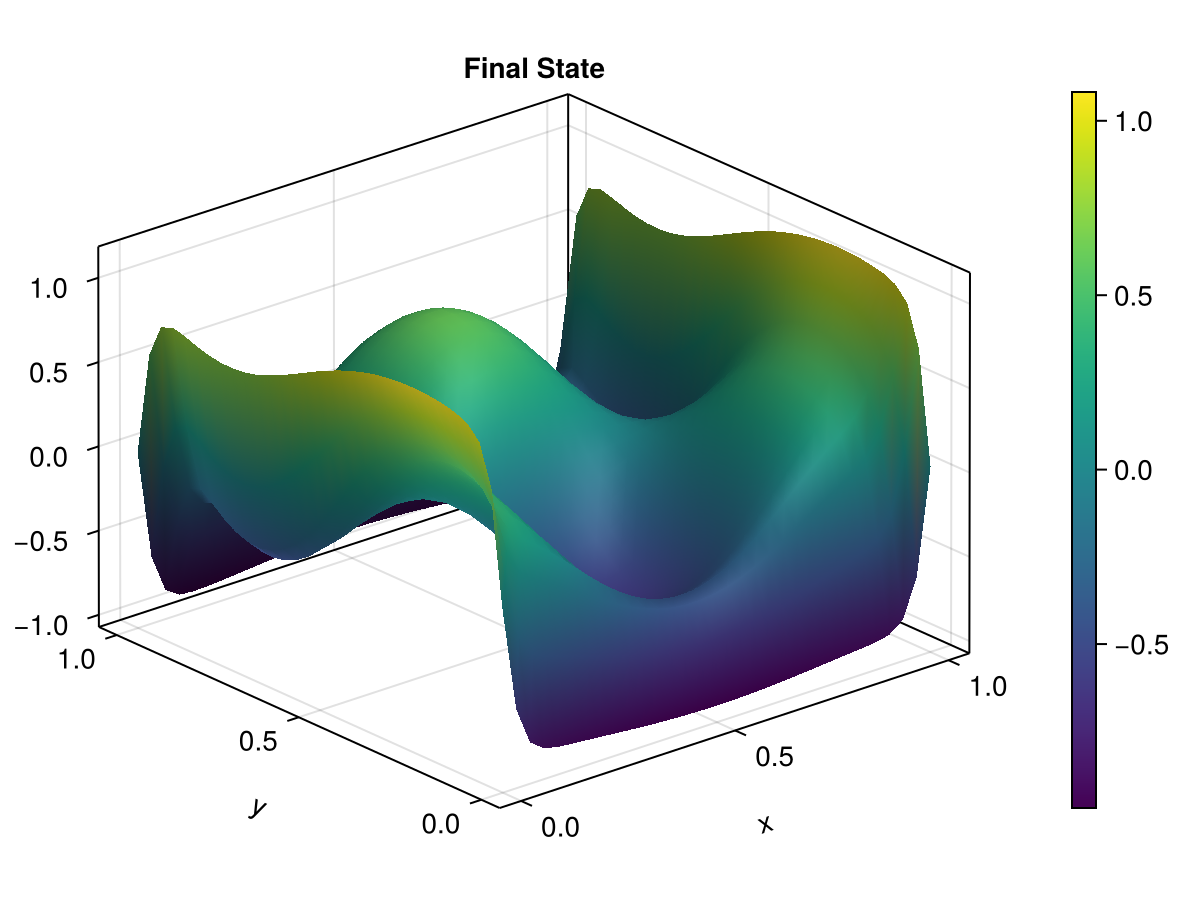

API

mutable struct AllenCahn2DModel <: AbstractModel

2D Allen-Cahn equation PDE Model

finite_diff_dirichlet_model(Nx, Ny, Δx, Δy, params)

finite_diff_model(model, params)

finite_diff_periodic_model(Nx, Ny, Δx, Δy, params)

integrate_model(tdata, u0; ...)
integrate_model(tdata, u0, input; kwargs...)

integrate_model_with_control_CNAB(
    tdata,
    u0,
    input;
    linear_matrix,
    cubic_matrix,
    control_matrix,
    const_stepsize,
    u3_jm1
)

integrate_model_with_control_SICN(
    tdata,
    u0,
    input;
    linear_matrix,
    cubic_matrix,
    control_matrix,
    const_stepsize
)

integrate_model_without_control_CNAB(
    tdata,
    u0;
    linear_matrix,
    cubic_matrix,
    const_stepsize,
    u3_jm1
)

integrate_model_without_control_SICN(
    tdata,
    u0;
    linear_matrix,
    cubic_matrix,
    const_stepsize
)