Bistable Nagumo equation

Overview

The bistable Nagumo equation (also called the Zeldovich equation or the asymmetric Allen-Cahn equation) is the scalar reaction-diffusion equation

\[u_t = \nu u_{xx} + u(u-a)(1-u), \qquad 0 < a < 1,\]

obtained from the FitzHugh-Nagumo system by dropping the recovery variable. It is one of the simplest PDEs whose reaction term is bistable: $f(u) = u(u-a)(1-u)$ has stable roots at $u=0$ and $u=1$ and an unstable root at the threshold $u=a$.

Some properties

Gradient flow: the equation is the $L_2$-gradient flow of the energy
\[E(u) = \int \left( \frac{\nu}{2} u_x^2 - F(u) \right) dx, \qquad F'(u) = f(u),\]
so $E$ decreases along every solution and all bounded trajectories converge to steady states.
Comparison principle: initial data with $u_0 \le a$ everywhere decays to zero. Escape from the zero state requires a positive excursion above $a$ that is both high and wide enough to overcome diffusion.
Threshold phenomenon: on a bounded domain with homogeneous Dirichlet conditions, for $a < 1/2$ and a domain larger than a saddle-node value $L^*(\nu, a)$ there are exactly three nonnegative steady states: the zero state, an unstable bump (the critical nucleus, with exactly one unstable eigendirection), and a stable plateau near $u \equiv 1$. The stable manifold of the critical nucleus separates the basin of attraction of $u \equiv 0$ from that of the plateau. This makes the model a convenient test case for methods that estimate regions of attraction.

Model

Expanding the reaction term as $u(u-a)(1-u) = -a u + (1+a) u^2 - u^3$, the Nagumo equation becomes a linear-quadratic-cubic model:

\[\dot{\mathbf{u}}(t) = \mathbf{Au}(t) + \mathbf{F}(\mathbf{u}(t) \oslash \mathbf{u}(t)) + \mathbf{E}(\mathbf{u}(t) \oslash \mathbf{u}(t) \oslash \mathbf{u}(t)) + \mathbf{Bw}(t)\]

where

$\mathbf{u}\in\mathbb{R}^N$: the state vector
$\mathbf{w}\in\mathbb{R}^m$: the input vector (boundary values)
$\mathbf{A}\in\mathbb{R}^{N\times N}$: the linear state matrix (diffusion and the $-au$ term)
$\mathbf{F}\in\mathbb{R}^{N\times N(N+1)/2}$: the quadratic state matrix without redundancy (the $(1+a)u^2$ term)
$\mathbf{E}\in\mathbb{R}^{N\times N(N+1)(N+2)/6}$: the cubic state matrix without redundancy (the $-u^3$ term)
$\mathbf{B}\in\mathbb{R}^{N\times m}$: the control input matrix

The model parameters are passed as params=Dict(:ν => ..., :a => ...).

Numerical Integration

For the numerical integration we consider two methods:

Semi-Implicit Crank-Nicolson (SICN)
Crank-Nicolson Adams-Bashforth (CNAB)

Both treat the linear operator $\mathbf{A}$ with Crank-Nicolson and the reaction term $\mathbf{N}(\mathbf{u}) = \mathbf{F}\mathbf{u}^{\langle 2\rangle} + \mathbf{E}\mathbf{u}^{\langle 3\rangle}$ explicitly.

SICN:

\[\mathbf{u}(t_{k+1}) = \left(\mathbf{I}-\frac{\Delta t}{2}\mathbf{A}\right)^{-1} \left\{ \left( \mathbf{I} + \frac{\Delta t}{2}\mathbf{A} \right)\mathbf{u}(t_k) + \Delta t\,\mathbf{N}(\mathbf{u}(t_k)) + \frac{\Delta t}{2} \mathbf{B}\left[ \mathbf{w}(t_{k+1}) + \mathbf{w}(t_k) \right]\right\}\]

CNAB:

If $k=1$ the SICN step is used. If $k\geq 2$

\[\mathbf{u}(t_{k+1}) = \left(\mathbf{I}-\frac{\Delta t}{2}\mathbf{A}\right)^{-1} \left\{ \left( \mathbf{I} + \frac{\Delta t}{2}\mathbf{A} \right)\mathbf{u}(t_k) + \frac{3\Delta t}{2}\mathbf{N}(\mathbf{u}(t_k)) - \frac{\Delta t}{2}\mathbf{N}(\mathbf{u}(t_{k-1})) + \frac{\Delta t}{2} \mathbf{B}\left[ \mathbf{w}(t_{k+1}) + \mathbf{w}(t_k) \right]\right\}\]

where $\mathbf{u}^{\langle 2 \rangle}=\mathbf{u} \oslash \mathbf{u}$ and $\mathbf{u}^{\langle 3 \rangle}=\mathbf{u} \oslash \mathbf{u} \oslash \mathbf{u}$.

The fast integrator integrate_model_fast uses the same schemes with a pre-built structured solver from build_fast_solver (FFT-based for periodic boundaries, eigendecomposition of the symmetric tridiagonal operator for Dirichlet and mixed boundaries).

!!! Note Please go over the derivations in 1D heat equation and Viscous Burgers' equation for details on how to construct each operators.

Example

using CairoMakie
using LinearAlgebra
using PolynomialModelReductionDataset
const pomoreda = PolynomialModelReductionDataset

# Setup
Ω = (0.0, 20.0)
T = (0.0, 40.0)
Nx = 2^8
dt = 1e-2
nagumo = pomoreda.NagumoModel(
    spatial_domain=Ω, time_domain=T, Δx=((Ω[2]-Ω[1]) + 1/Nx)/Nx, Δt=dt,
    params=Dict(:ν => 1.0, :a => 0.3), BC=:dirichlet
)
DS = 10
x = nagumo.xspan
xc = 0.5 * (Ω[1] + Ω[2])

# Operators and fast solver
A, F, E, B = nagumo.finite_diff_model(nagumo, nagumo.params)
solver = pomoreda.build_fast_solver(nagumo, nagumo.params; scheme=:CN)

# Two Gaussian bumps on either side of the threshold
nagumo.IC = 0.25 * exp.(-((x .- xc) / 4.0).^2)
U_small = pomoreda.integrate_model_fast(nagumo, solver, nagumo.tspan, nagumo.IC;
                                        quadratic_matrix=F, cubic_matrix=E, integrator_type=:CNAB)
nagumo.IC = 1.0 * exp.(-((x .- xc) / 4.0).^2)
U_large = pomoreda.integrate_model_fast(nagumo, solver, nagumo.tspan, nagumo.IC;
                                        quadratic_matrix=F, cubic_matrix=E, integrator_type=:CNAB)

fig = Figure(size=(900, 400))
ax1 = Axis(fig[1, 1], xlabel=L"x", ylabel=L"t", title="Small bump: decays to 0")
heatmap!(ax1, x, nagumo.tspan[1:DS:end], U_small[:, 1:DS:end], colorrange=(0, 1))
ax2 = Axis(fig[1, 2], xlabel=L"x", ylabel=L"t", title="Large bump: escapes to the plateau")
hm = heatmap!(ax2, x, nagumo.tspan[1:DS:end], U_large[:, 1:DS:end], colorrange=(0, 1))
Colorbar(fig[1, 3], hm)
fig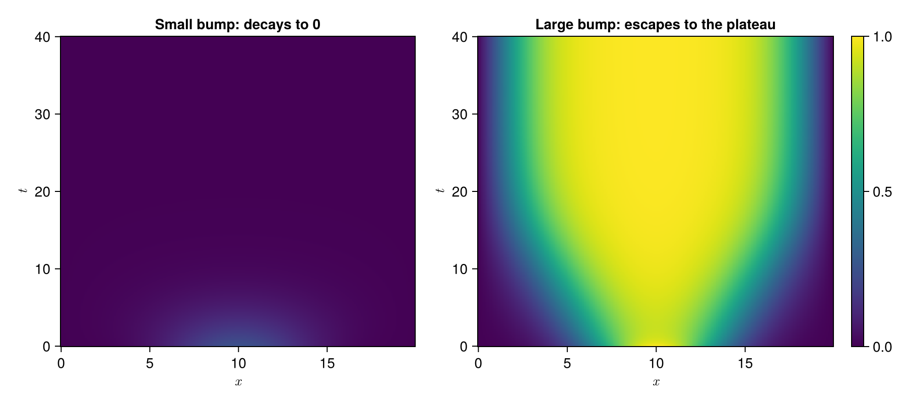

API

PolynomialModelReductionDataset.Nagumo.NagumoModel — Type

mutable struct NagumoModel <: AbstractModel

Bistable Nagumo equation model (also called the Zeldovich or asymmetric Allen-Cahn equation). It is the scalar FitzHugh-Nagumo equation without the recovery variable:

\[\frac{\partial u}{\partial t} = \nu\frac{\partial^2 u}{\partial x^2} + u(u-a)(1-u)\]

where $u$ is the state variable, $ν$ is the diffusion coefficient, and $a \in (0,1)$ is the threshold parameter. Expanding the reaction term,

\[u(u-a)(1-u) = -a u + (1+a) u^2 - u^3,\]

so the semi-discrete model is linear-quadratic-cubic in the state. The reaction term has stable roots at $u=0$ and $u=1$ and an unstable root at $u=a$. For $a<1/2$ and a large enough Dirichlet domain the zero state is locally but not globally stable: a nontrivial unstable steady state (the critical nucleus) separates the basin of $u\equiv 0$ from that of the plateau state near $u\equiv 1$.

Fields

spatial_domain::Tuple{Real,Real}: spatial domain
time_domain::Tuple{Real,Real}: temporal domain
param_domain::Dict{Symbol,Tuple{Real,Real}}: parameter domain
Δx::Real: spatial grid size
Δt::Real: temporal step size
xspan::Vector{<:Real}: spatial grid points
tspan::Vector{<:Real}: temporal points
params::Dict{Symbol,Union{Real,AbstractArray{<:Real}}}: parameters (:ν diffusion, :a threshold)
spatial_dim::Int: spatial dimension
time_dim::Int: temporal dimension
param_dim::Dict{Symbol,Int}: parameter dimension
IC::AbstractArray{<:Real}: initial condition
BC::Symbol: boundary condition
finite_diff_model::Function: model using Finite Difference
integrate_model::Function: integrator using Crank-Nicolson (linear) Explicit (nonlinear) method